

Keras Internals: Debugging a Softmax Behavior Inconsistency
Exploring the Keras Softmax implementation details and fixing a subtle behavior inconsistency with masking.

As an engineer on the Keras team, I often encounter interesting technical details. Since Keras is an open-source project, I have the opportunity to share some of these insights with the community.
For the uninitiated, Keras is a multi-backend deep learning library. It provides a powerful, and easy to use API on top of a variety of backends, such as JAX, PyTorch, and TensorFlow.

Recently, a behavioral discrepancy was identified between the Keras Softmax implementation, particularly when using input masking, and its counterpart in JAX. Ensuring consistent behavior across different computational backends (such as JAX, TensorFlow, and PyTorch) is a fundamental requirement for a multi-backend framework like Keras.
As a part of the investigation I ended up peeking into the internals of how Keras implements Softmax, and it was interesting to see the design choices made to accommodate a multi-backend API.
Softmax Primer
Let’s take a small primer on what the softmax function does and how the mask argument changes its behavior. Then we can discuss the behavioral inconsistencies that the Softmax implementation was exhibiting.
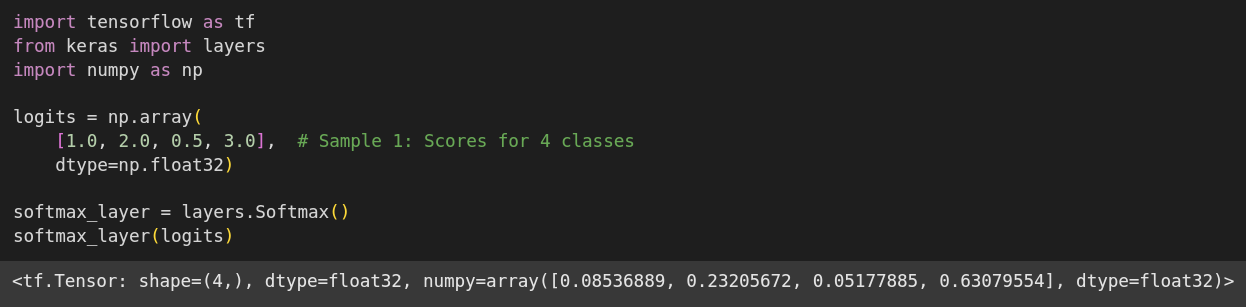
Softmax is a function commonly used in the final layer of neural networks for classification tasks.
It takes a vector of arbitrary real-valued scores (often called logits) and transforms them into a probability distribution.
Essentially, it converts these scores into probabilities that sum up to 1, where each probability corresponds to the likelihood of a particular class.
Higher input scores result in higher output probabilities.
Mask
The mask argument adds a layer of control. It allows you to specify which elements of the input vector should be included in the softmax calculation. When an element is masked (typically indicated by False in the mask array), it's effectively excluded from the probability calculation.
In practice, this is often achieved by assigning a very large negative value to the masked elements before applying the exponential function. This ensures their contribution to the final probability distribution is zero (or numerically very close to zero), and the remaining probabilities are normalized across only the unmasked elements.
Behavior Divergence with JAX
GitHub issue: Softmax layer diverges from jax.nn.softmax · Issue #21123 · keras-team/keras · GitHub
What happens when someone masks an entire axis while calculating the softmax, any guesses?
Let’s look at the code.
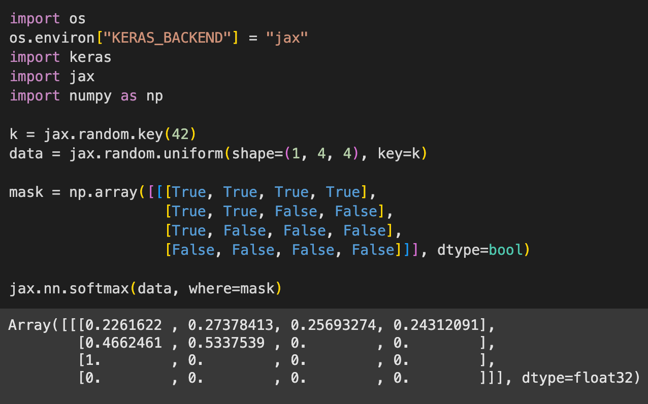
We create a random tensor sampled from a uniform random distribution, of shape
(1, 4, 4).We define a boolean mask, with one of the axes completely masked out (all positions set to
False)Calculate the softmax activation for the tensor with the default axis (-1) and pass the mask as an argument to the
whereparameter of thejax.nn.softmaxfunction.As you might guess, we get a softmax projection of the original tensor, where each numeric in its respective axis represents a probability. All the logits across an axis must sum up to 1.
Also notice that the masked inputs are all zeroed out, as one might expect.
Let’s try to recreate this operation with the same input tensor and mask, while using Keras with JAX backend.
We start by initializing a softmax layer (again on the default axis, -1)
We pass the random tensor to the layer, along with the mask
The outputs look similar, except for the last row. For some reason instead of being zeroed out, all the elements are set to 0.25!
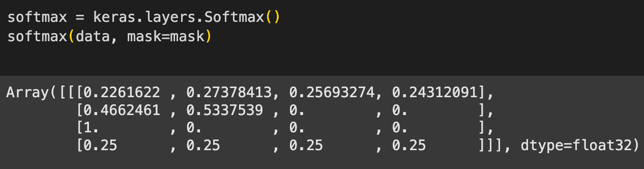
Why do you think that is? Hint, it has something to do with how masking is implemented. If you look closely, returning 0.25 across all the four masked positions is similar to returning a uniform probability distribution over the entire axis (each position has the same probability).
There is no hard guidance around what the output of a softmax layer should look like when using masking, and it’s interesting to see this behavior discrepancy between JAX and Keras when masking an entire axis.
It’s not possible to contrast these outputs with TensorFlow or PyTorch, since their softmax implementations do not support masking. A natural choice at this point is to treat the JAX softmax behavior as canonical, and ensure Keras follows it.
How Keras implements Softmax
Let’s understand the backend agnostic softmax implementation which keras provides. Often, each backend may differ slightly in the APIs it offers, leading to some interesting design choices.
Let’s analyze the call() method of keras.layers.Softmax, since that’s where the interesting stuff happens. I’ve added comments to the function to explain all the details.
![def call(self, inputs, mask=None): # This method defines the forward pass of the Softmax layer. # It takes the input tensor and an optional mask. if mask is not None: # This block executes only if a mask is provided. # The mask indicates which elements should be considered (True) # and which should be ignored (False) in the softmax calculation. # Create an 'adder' tensor to modify the inputs based on the mask. adder = ( # 1. Cast the boolean mask to the same dtype as inputs (e.g., float32). # True becomes 1.0, False becomes 0.0. # 2. Subtract from 1.0: This inverts the values. # Elements to keep (originally True/1.0) become 0.0. # Elements to mask out (originally False/0.0) become 1.0. (1.0 - backend.cast(mask, inputs.dtype)) # 3. Multiply by a large negative number. # Elements to keep (0.0) remain 0.0. # Elements to mask out (1.0) become a large negative number. * _large_negative_number(inputs.dtype) # `_large_negative_number` provides a dtype-appropriate large negative value # to ensure numerical stability when exponentiated later. ) # Add the 'adder' to the original inputs. # - For elements to keep, inputs = inputs + 0.0 (no change). # - For elements to mask out, inputs = inputs + large_negative_number. # This effectively drives the logits of masked elements towards -infinity. inputs += adder # Check if the softmax axis is specified as a tuple or list (potentially multi-axis). if isinstance(self.axis, (tuple, list)): # If more than one axis is specified for softmax calculation. if len(self.axis) > 1: # Keras provides its own implementation for multi-axis softmax # using the logsumexp trick for numerical stability. # Formula: softmax(x) = exp(x - logsumexp(x)) # # WHY IMPLEMENT MANUALLY? Backend Compatibility: # This manual implementation is necessary because native multi-axis # softmax is not supported by all backends (specifically TensorFlow # and PyTorch, although JAX *does* support it). # By implementing it here, Keras ensures consistent behavior and # provides this extended functionality across all supported backends, # saving users from implementing it themselves per backend. return backend.numpy.exp( inputs - backend.math.logsumexp( inputs, axis=self.axis, keepdims=True # Keep dimensions for broadcasting ) ) # If self.axis is a tuple/list but contains only one axis. else: # Delegate to the standard backend softmax implementation for a single axis. # `activations.softmax` calls the appropriate backend function (JAX, TF, PyTorch). return activations.softmax(inputs, axis=self.axis[0]) # Extract the single axis # If self.axis is just an integer (standard single-axis case). # Delegate to the standard backend softmax implementation. return activations.softmax(inputs, axis=self.axis)](https://substackcdn.com/image/fetch/$s_!1ZVc!,f_auto,q_auto:good,fl_progressive:steep/https%3A%2F%2Fsubstack-post-media.s3.amazonaws.com%2Fpublic%2Fimages%2Fb29aba2b-e7a5-49bb-91cc-f7c6478cd1a0_3608x5472.png "def call(self, inputs, mask=None): # This method defines the forward pass of the Softmax layer. # It takes the input tensor and an optional mask. if mask is not None: # This block executes only if a mask is provided. # The mask indicates which elements should be considered (True) # and which should be ignored (False) in the softmax calculation. # Create an 'adder' tensor to modify the inputs based on the mask. adder = ( # 1. Cast the boolean mask to the same dtype as inputs (e.g., float32). # True becomes 1.0, False becomes 0.0. # 2. Subtract from 1.0: This inverts the values. # Elements to keep (originally True/1.0) become 0.0. # Elements to mask out (originally False/0.0) become 1.0. (1.0 - backend.cast(mask, inputs.dtype)) # 3. Multiply by a large negative number. # Elements to keep (0.0) remain 0.0. # Elements to mask out (1.0) become a large negative number. * _large_negative_number(inputs.dtype) # `_large_negative_number` provides a dtype-appropriate large negative value # to ensure numerical stability when exponentiated later. ) # Add the 'adder' to the original inputs. # - For elements to keep, inputs = inputs + 0.0 (no change). # - For elements to mask out, inputs = inputs + large_negative_number. # This effectively drives the logits of masked elements towards -infinity. inputs += adder # Check if the softmax axis is specified as a tuple or list (potentially multi-axis). if isinstance(self.axis, (tuple, list)): # If more than one axis is specified for softmax calculation. if len(self.axis) > 1: # Keras provides its own implementation for multi-axis softmax # using the logsumexp trick for numerical stability. # Formula: softmax(x) = exp(x - logsumexp(x)) # # WHY IMPLEMENT MANUALLY? Backend Compatibility: # This manual implementation is necessary because native multi-axis # softmax is not supported by all backends (specifically TensorFlow # and PyTorch, although JAX *does* support it). # By implementing it here, Keras ensures consistent behavior and # provides this extended functionality across all supported backends, # saving users from implementing it themselves per backend. return backend.numpy.exp( inputs - backend.math.logsumexp( inputs, axis=self.axis, keepdims=True # Keep dimensions for broadcasting ) ) # If self.axis is a tuple/list but contains only one axis. else: # Delegate to the standard backend softmax implementation for a single axis. # `activations.softmax` calls the appropriate backend function (JAX, TF, PyTorch). return activations.softmax(inputs, axis=self.axis[0]) # Extract the single axis # If self.axis is just an integer (standard single-axis case). # Delegate to the standard backend softmax implementation. return activations.softmax(inputs, axis=self.axis)")
Note: Keras uses a
backendobject whenever it wants to delegate computation to a backend-specific API. The backend object encapsulates the user-selected backend (JAX, TF, PyTorch). This allows all implementations to rely on a simple backend-based abstraction, without having to worry about how each computational backend handles a specific task.
Adding Masks
The intuition behind how softmax masking is implemented is simple. We add a very large negative number to all the masked positions; effectively negating their contribution to the softmax computation (since the probability of now choosing them is so low, that it’s practically zero). Therefore, numerically, they no longer contribute to the probability distribution.
Calculating Softmax over multiple Axes
An interesting detail is that while JAX supports multi-axis softmax, TensorFlow and PyTorch don’t. Therefore keras provides its own implementation for this case.
This is another cool reason to use keras, you get additional bells and whistles on top of functionality you already understand well, without requiring you to implement it yourself.
We use something called the log-sum-exp trick to calculate the softmax projection over multiple axes.
I won’t being going very deep into the mathematical derivation (even though it’s quite simple) for why this trick works in this article, because to-be-fair, I’m not the best math-guy out there (yet) to confidently be able to write derivations in my substack articles. However, I’ll nudge you towards an excellent article (< 4 min read) which gives you a solid mathematical grounding for this. You can find it here.
All the backends already support the logsumexp operation natively, which means this computation will be hardware-accelerated and well-optimized.
Implementing the logsumexp trick
backend.math.logsumexp(inputs, axis=self.axis, keepdims=True)This calculates
log(sum(exp(inputs)))across the specified axis (or axes).
Crucially, the
logsumexpfunction itself is implemented internally in a numerically stable way, often by subtracting the maximum value before exponentiating:logsumexp(x) = max(x) + log(sum(exp(x - max(x)))). This prevents the intermediate exp calculations from overflowing. Note, the article I linked above derives this too.axis=self.axis: Tells the function which dimension(s) to sum over.keepdims=True: When summing over an axis (or axes), that dimension usually disappears (since we reduce over it).keepdims=Trueensures that the summed axes are retained with a size of 1. This makes the shape of the logsumexp result compatible for broadcasting when subtracted from the original inputs tensor.
inputs - backend.math.logsumexp(...)This performs the subtraction
inputs - log(sum(exp(inputs))). Because logsumexp's result was computed stably and has compatible dimensions (due tokeepdims=True), this subtraction is well-defined.The values here are essentially the logarithms of the final softmax probabilities.
backend.numpy.exp(...)This takes the exponent of the result from the previous step, effectively converting the stable log-probabilities back into the actual softmax probabilities:
exp(log(softmax(inputs))) = softmax(inputs).
In case of a single-axis softmax computation, we simply call the activations.softmax(…) method. It internally calls keras.ops.softmax(x, axis=axis).
Let’s understand how that’s implemented. As earlier, I’ve added comments to all the lines
![def softmax(x, axis=-1): # Check if the specified 'axis' is an integer AND if the dimension size along that axis is 1. if isinstance(axis, int) and x.shape[axis] == 1: # Issue a warning if softmax is applied on an axis with size 1. warnings.warn( f"You are using a softmax over axis {axis} " f"of a tensor of shape {x.shape}. This axis " "has size 1. The softmax operation will always return " "the value 1, which is likely not what you intended. " "Did you mean to use a sigmoid instead?" ) # Check if the input tensor 'x' (or any others if passed in the tuple) is a symbolic tensor. if any_symbolic_tensors((x,)): # If symbolic, delegate the operation to the symbolic execution path of the Softmax layer/op. return Softmax(axis).symbolic_call(x) # Check if the 'axis' argument is a tuple (indicating multi-axis softmax). # Note: We don't enter this if-condition when using keras.layers.Softmax, since this case is # explicitly handled already (as we discussed above). if isinstance(axis, tuple): # Create a list of axis indices that are *not* included in the 'axis' tuple. axis_to_keep = [v for v in range(len(x.shape)) if v not in axis] # Transpose the input tensor 'x' to bring all axes specified in 'axis' to the end. x_transposed = backend.numpy.transpose(x, axes=(*axis_to_keep, *axis)) # Reshape the transposed tensor: group 'axis_to_keep' dimensions and flatten 'axis' dimensions into one. x_reshaped = backend.numpy.reshape( x_transposed, # Target shape: keep original sizes for 'axis_to_keep', combine 'axis' dimensions (-1 infers size). (*[x.shape[v] for v in axis_to_keep], -1) ) # Apply the backend's native softmax function along the last axis (-1) of the reshaped tensor. x = backend.nn.softmax(x_reshaped, axis=-1) # Reshape the result back to the shape it had after the initial transpose operation. x = backend.numpy.reshape(x, x_transposed.shape) # Transpose the tensor back to its original axis order by finding the inverse permutation. x = backend.numpy.transpose( # The tensor to transpose back. x, # Calculate the inverse permutation: create the transposed order, argsort finds the original positions. axes=list(backend.numpy.argsort([*axis_to_keep, *axis])) ) return x else: # Directly call the backend's native softmax implementation for a single axis. return backend.nn.softmax(x, axis=axis)](https://substackcdn.com/image/fetch/$s_!GGqJ!,f_auto,q_auto:good,fl_progressive:steep/https%3A%2F%2Fsubstack-post-media.s3.amazonaws.com%2Fpublic%2Fimages%2Fd02f598e-d2e8-4243-974a-b84bc922acc6_4289x4380.png "def softmax(x, axis=-1): # Check if the specified 'axis' is an integer AND if the dimension size along that axis is 1. if isinstance(axis, int) and x.shape[axis] == 1: # Issue a warning if softmax is applied on an axis with size 1. warnings.warn( f\"You are using a softmax over axis {axis} \" f\"of a tensor of shape {x.shape}. This axis \" \"has size 1. The softmax operation will always return \" \"the value 1, which is likely not what you intended. \" \"Did you mean to use a sigmoid instead?\" ) # Check if the input tensor 'x' (or any others if passed in the tuple) is a symbolic tensor. if any_symbolic_tensors((x,)): # If symbolic, delegate the operation to the symbolic execution path of the Softmax layer/op. return Softmax(axis).symbolic_call(x) # Check if the 'axis' argument is a tuple (indicating multi-axis softmax). # Note: We don't enter this if-condition when using keras.layers.Softmax, since this case is # explicitly handled already (as we discussed above). if isinstance(axis, tuple): # Create a list of axis indices that are *not* included in the 'axis' tuple. axis_to_keep = [v for v in range(len(x.shape)) if v not in axis] # Transpose the input tensor 'x' to bring all axes specified in 'axis' to the end. x_transposed = backend.numpy.transpose(x, axes=(*axis_to_keep, *axis)) # Reshape the transposed tensor: group 'axis_to_keep' dimensions and flatten 'axis' dimensions into one. x_reshaped = backend.numpy.reshape( x_transposed, # Target shape: keep original sizes for 'axis_to_keep', combine 'axis' dimensions (-1 infers size). (*[x.shape[v] for v in axis_to_keep], -1) ) # Apply the backend's native softmax function along the last axis (-1) of the reshaped tensor. x = backend.nn.softmax(x_reshaped, axis=-1) # Reshape the result back to the shape it had after the initial transpose operation. x = backend.numpy.reshape(x, x_transposed.shape) # Transpose the tensor back to its original axis order by finding the inverse permutation. x = backend.numpy.transpose( # The tensor to transpose back. x, # Calculate the inverse permutation: create the transposed order, argsort finds the original positions. axes=list(backend.numpy.argsort([*axis_to_keep, *axis])) ) return x else: # Directly call the backend's native softmax implementation for a single axis. return backend.nn.softmax(x, axis=axis)")
After some initial validation, we check whether we’re operating over symbolic tensors (when no actual inputs have been provided) and handle those accordingly.
We check whether we are computing softmax over a single axis, or over multiple axes. We won’t hit this branch in our case, since we already handled that at the Softmax Layer level (as discussed above). It’s still interesting to see how this is implemented.
The gist is that we temporarily rearrange and flatten the specific axes we’re interested in into a single dimension at the end. We then apply the standard single-axis softmax to this flattened dimension before reversing the rearrangement to restore the original tensor shape.The last else condition is what we’ll usually be dealing with in case of
keras.layers.Softmax. It delegates the single-axis softmax calculation to the respective backend that we might be using.
The Masking inconsistency
That was a lot about how Keras implements Softmax. Now let’s try and understand why keras outputs a uniform probability distribution when we mask an an entire axis.
We’ll need to go back to how masking is implemented. We add a large number to all masked positions to drop their contribution to the probability distribution to practically zero when compared to all other positions.
But what happens when we do this at all the positions across a softmax axis?
Driving all logits towards negative infinity makes them numerically indistinguishable from each other. When softmax exponentiates these similar, large negative inputs, the outputs become tiny, near-identical positive numbers. Normalizing these values inevitably leads to an equal probability assigned to each position – a uniform distribution.
The Fix
It’s quite easy to fix this issue once you know why it happens. All we need to do is to multiply the final outputs, whatever they are, with the original boolean mask. This ensures that all the masked outputs are always set to zero.
The following figure shows you how we need to modify the existing implementation.
![def call(self, inputs, mask=None): if mask is not None: adder = ( 1.0 - backend.cast(mask, inputs.dtype) ) * _large_negative_number(inputs.dtype) inputs += adder if isinstance(self.axis, (tuple, list)): if len(self.axis) > 1: outputs = backend.numpy.exp( inputs - backend.math.logsumexp( inputs, axis=self.axis, keepdims=True ) ) else: outputs = activations.softmax(inputs, axis=self.axis[0]) else: outputs = activations.softmax(inputs, axis=self.axis) if mask is not None: # Apply the mask to the softmax output to ensure that masked # values are set to 0 in case the entire axis is masked. outputs = backend.numpy.multiply( outputs, backend.cast(mask, outputs.dtype) ) return outputs](https://substackcdn.com/image/fetch/$s_!ZKif!,f_auto,q_auto:good,fl_progressive:steep/https%3A%2F%2Fsubstack-post-media.s3.amazonaws.com%2Fpublic%2Fimages%2Fa4f7da56-5c08-4892-9023-8d73b46e0e45_814x605.png "def call(self, inputs, mask=None): if mask is not None: adder = ( 1.0 - backend.cast(mask, inputs.dtype) ) * _large_negative_number(inputs.dtype) inputs += adder if isinstance(self.axis, (tuple, list)): if len(self.axis) > 1: outputs = backend.numpy.exp( inputs - backend.math.logsumexp( inputs, axis=self.axis, keepdims=True ) ) else: outputs = activations.softmax(inputs, axis=self.axis[0]) else: outputs = activations.softmax(inputs, axis=self.axis) if mask is not None: # Apply the mask to the softmax output to ensure that masked # values are set to 0 in case the entire axis is masked. outputs = backend.numpy.multiply( outputs, backend.cast(mask, outputs.dtype) ) return outputs")
Conclusion
We went over how Keras implements the softmax layer, and how sometimes computational tricks can lead to unexpected results! It’s often not hard to fix these issues if you truly understand how things are implemented under the hood.
See you in the next one!